LLM-driven evolutionary search is a powerful approach for discovering algorithms and designs, but existing frameworks are difficult to extend and compare.
We introduce SkyDiscover, a flexible and modular framework for AI-driven scientific and algorithmic discovery. We use it to build two adaptive evolutionary algorithms about 2.5K LoC and set SOTA results 200+ tasks:
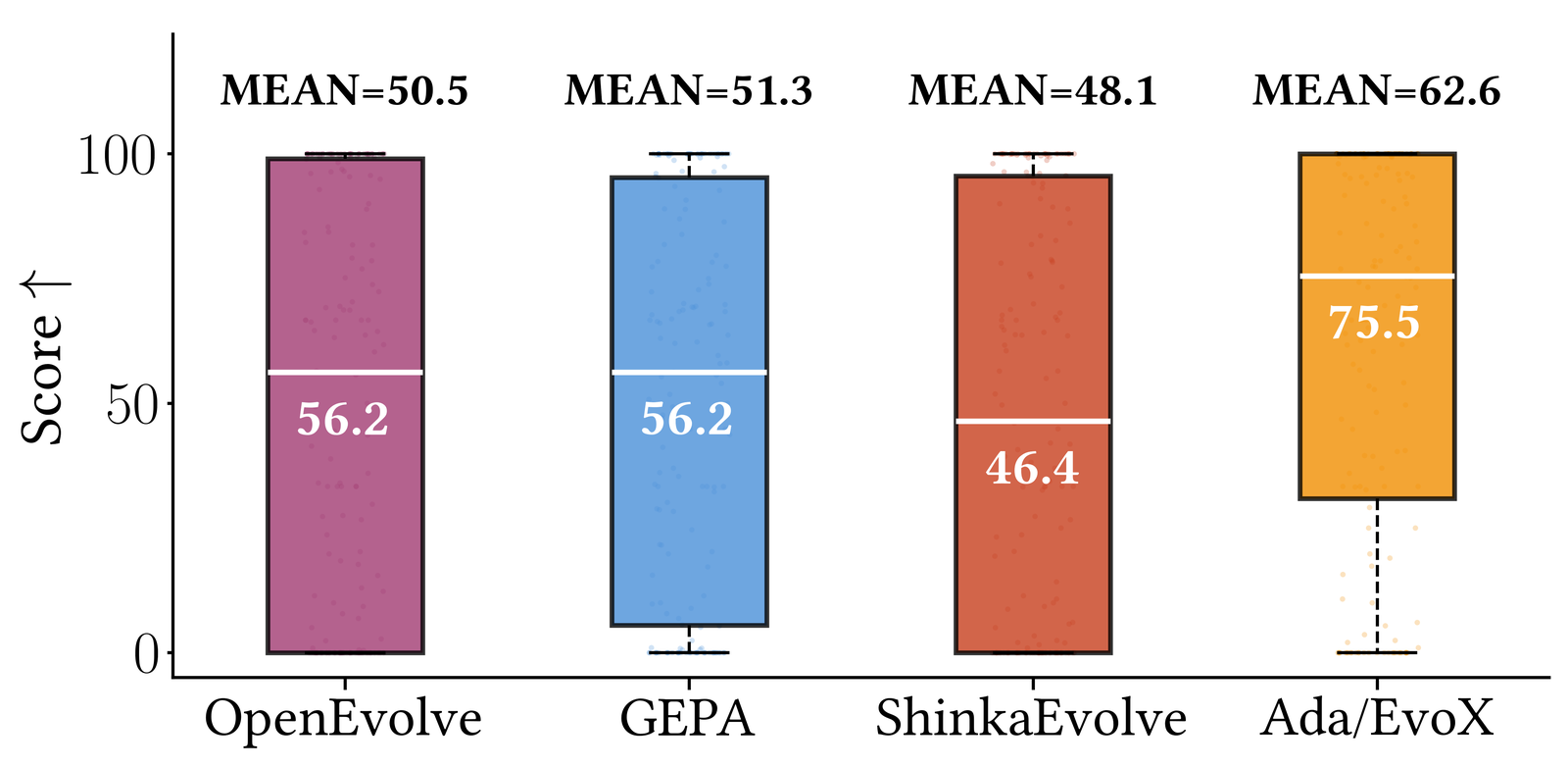
- 🏆 Best open-source performance: improving median scores by ~34% on 172 Frontier-CS programming problems over OpenEvolve, GEPA, and ShinkaEvolve.
- 💪 Matching or exceeding AlphaEvolve and human SOTA: on 6/8 math and 6/6 systems optimization tasks.
- 🚀 Concrete discoveries with real impact: 41% lower cross-cloud transfer cost, 14% better GPU load balance for MoE serving, and 29% lower KV-cache pressure via GPU model placement.
Background: The Rise of AI-Driven Discovery
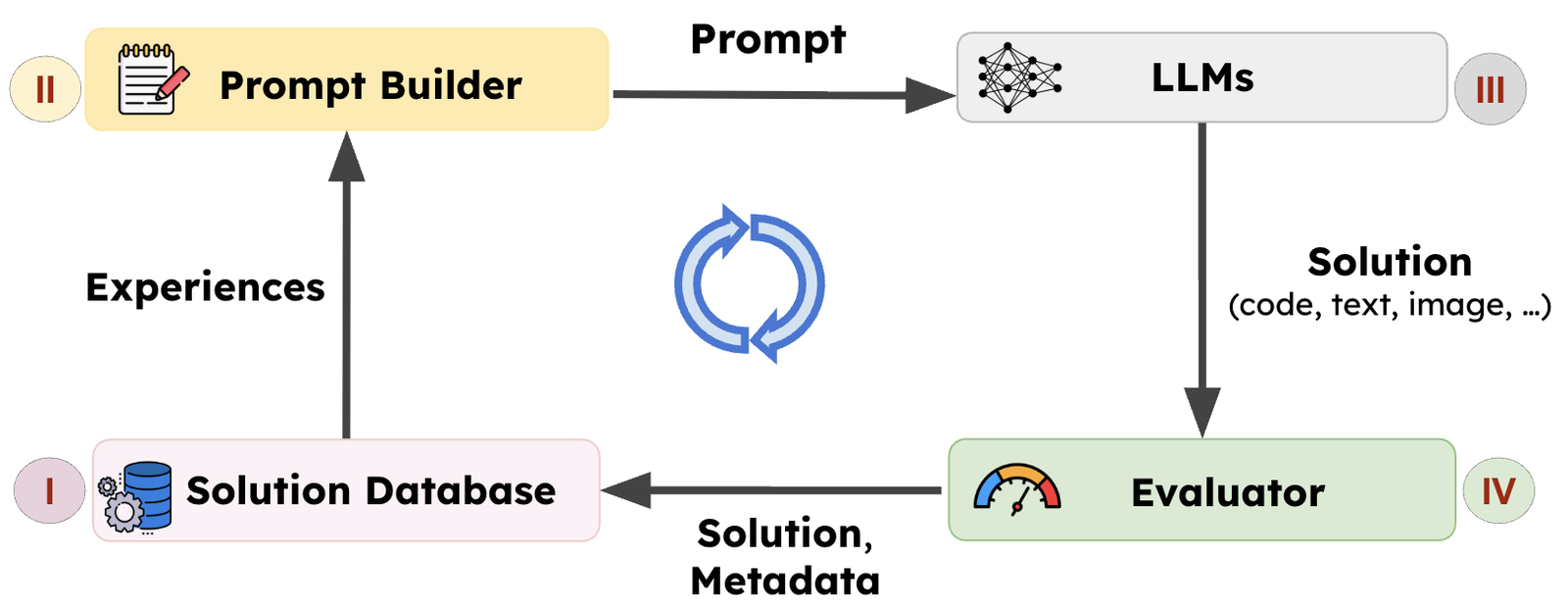
A defining capability of intelligent systems is the ability to learn from experience. One powerful paradigm is LLM-driven search, pioneered by AlphaEvolve. In this approach, the system maintains a (I) population of prior solutions, uses them to (II) construct experience-informed prompts, (III) generates new candidates, and (IV) evaluates them. The resulting solutions and metadata are added back to the population, forming a closed improvement loop.
Frameworks such as AlphaEvolve, OpenEvolve, GEPA, and ShinkaEvolve have demonstrated the promise of this paradigm. AlphaEvolve discovered improved matrix multiplication algorithms and enabled data center scheduling optimizations at Google, while GEPA learned reusable agent skills and optimized agent architectures across domains. Together, these results establish LLM-driven search as a powerful approach for scientific and algorithmic discovery.
Challenge
Although existing systems share a similar high-level loop, their implementations are tightly coupled and difficult to extend. For example, OpenEvolve uses MAP-Elites–based selection in the solution database with fixed prompt templates; GEPA couples Pareto-front selection with recombination and mutation operators in prompt construction. As a result, modifying a single component such as introducing a new strategy often requires rewriting core infrastructure.
SkyDiscover: A Flexible Framework for AI-driven Scientific and Algorithmic Discovery
To address these limitations, we built SkyDiscover, a modular and flexible framework for AI-driven discovery, designed around two key goals:
- Generality: Support diverse algorithms and enable unified evaluation on shared benchmarks.
- Flexibility: Enable rapid implementation and evaluation of new discovery techniques without modifying a monolithic system.
Architecture
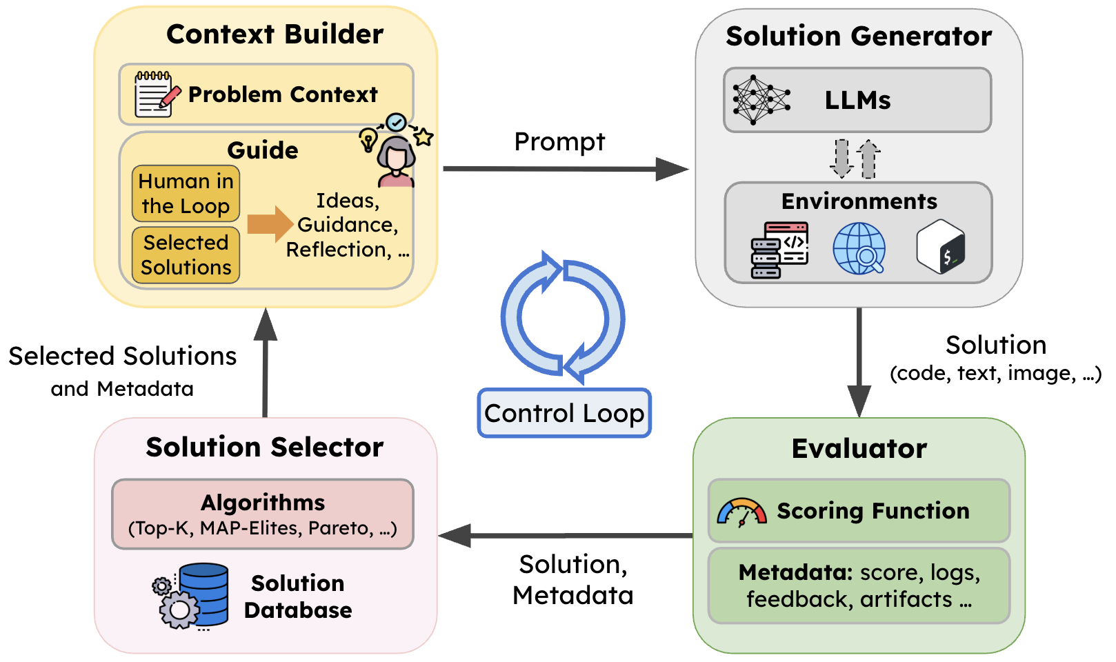
SkyDiscover preserves the same high-level evolutionary loop as in prior systems, but decouples each stage into reusable components and makes the control logic itself programmable.
- Context Builder. Constructs prompts by combining the problem context with knowledge accumulated from prior solutions (e.g., including reflections and feedback).
- Solution Generator. Produces candidate solutions via LLM calls and optional tool use.
- Evaluator. Scores candidate solutions and logs feedback into the solution database for future iterations.
- Solution Selector. Maintains the solution pool and chooses which prior solutions guide the next iteration (e.g., random, Top-K, MAP-Elites, Pareto).
- Flexible control loop: enables independent orchestration of these four components above. This enables the implementation of the two SOTA adaptive algorithms as we will discuss next.
New Discovery Algorithms Built on SkyDiscover
SkyDiscover’s modular components make it easy to implement and compare discovery methods under identical budgets and models. Using this, we developed two adaptive evolutionary algorithms:
- AdaEvolve, which dynamically adjusts its optimization behavior based on observed progress.
- EvoX, which dynamically evolves the optimization (evolution) strategy itself using LLMs on the fly.
Across 200+ tasks in mathematical optimization, systems design, and Frontier-CS programming, under a fixed budget of 100 candidate generations and fixed models (e.g., GPT-5, Gemini-3.0-Pro), AdaEvolve and EvoX deliver the strongest open-source performance we evaluated, outperforming OpenEvolve, GEPA, and ShinkaEvolve.
Mathematical Optimization
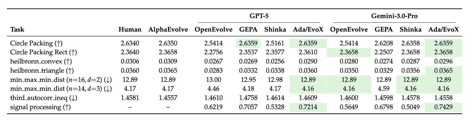
Across all 8 mathematical optimization tasks, Ada/EvoX achieves the best performance among all evaluated LLM frameworks. When compared to the state-of-the-art AlphaEvolve, we match or exceed its results in 6 out of 8 tasks. Specifically, the best achieved results beat AlphaEvolve in 3 tasks (Circle Packing, Circle Packing Rect, 3D min-max distance).
Systems Optimization
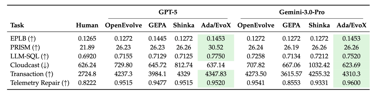
Across all 6 system optimization tasks, Ada/EvoX achieves the best performance among all evaluated LLM frameworks and beats existing human SOTA algorithms on 6 out of 6 tasks. The best solutions achieve, for example, 41% lower cloud transfer cost, 14% better GPU load balance for MoE serving, and 29% lower KV-cache pressure for GPU model placement.
Algorithmic Challenges
Evaluated on 172 Frontier-CS open-ended problems, Ada/EvoX achieves the highest performance among open-source discovery methods with a mean score of 62.6 and a median of 75.5. This represents mean and median improvements of 24% and 34% over OpenEvolve, 22% and 34% over GEPA, and 30% and 63% over ShinkaEvolve.
How Do These Two Discovery Algorithms Work?
We now provide overview of the two new algorithms built on top of SkyDiscover.
We’ll be sharing follow-up posts in the coming weeks that dive deeper into how each algorithm works under the hood!
#1: AdaEvolve: Progress-Aware Guidance for Discovery
Most discovery systems rely on fixed strategies (e.g., static exploration rates, rigid temperatures, fixed prompt templates), which often waste compute when discovery dynamics change. The optimization process searching for better solutions should account for these dynamics. In the domain of continuous optimization, adaptive gradient methods like AdaGrad and Adam tackles these issues by dynamically adjusting learning rates adaptively using the moments of gradients. However, for LLM based discovery, which is a zeroth order (gradient-free) optimization process, we need new formulations to rethink how we adapt the search dynamics.
AdaEvolve treats discovery as a non-stationary optimization process, dynamically adjusting search behavior as a function of observed progress and improvement signals.
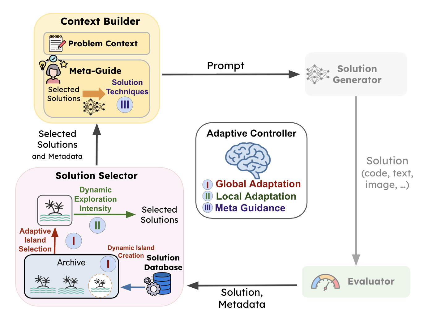
AdaEvolve operates through three levels of adaptation:
- Global Adaptation: Maintains multiple subpopulations (islands) and dynamically creates new islands or reallocates compute across islands using bandit-based scheduling.
- Local Adaptation: Adjusts the exploration–exploitation balance within each island population.
- Meta-Guidance: Introduces new solution techniques when progress stalls.
Collectively, these mechanisms allow AdaEvolve to continuously reshape the discovery strategy in response to observed search dynamics. Check out the paper for more details.
#2: EvoX: Meta-Evolving the Optimization Strategy
EvoX takes this idea one step further and asks the question: what if the strategy of how we select and present (learn) past experiences could be improved on the fly?
EvoX introduces Meta-Evolution. Instead of relying on manual designs, EvoX treats experience management as an evolvable program, continuously rewriting its own search code to adapt to each stage of discovery.
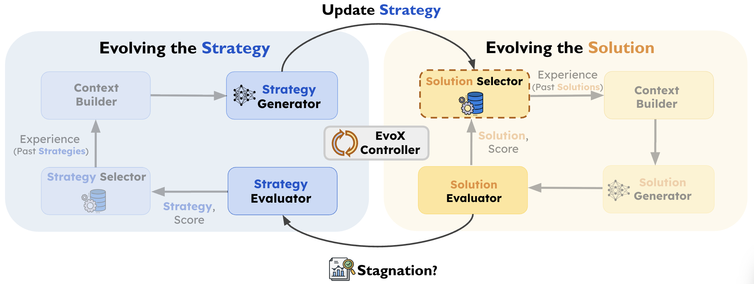
EvoX frames discovery as a multi-level system operating through two coupled loops:
- Solution Evolution (The What): Iteratively improving candidate solutions (the actual math or code designs) using the currently active search strategy.
- Strategy Evolution (The How): When plateau, EvoX uses an LLM to generate a new search strategy based on prior successes and the current state of the population.
The new strategy dynamically redefines which past solutions to select and what to do with them (e.g., local refinement, structural variation, or combining useful ideas). This allows EvoX to autonomously transition through different phases of discovery exactly when the problem demands it. Check out the paper for more details.
Case Studies: Discoveries Across Domains
We highlight representative solutions discovered by AdaEvolve and EvoX across diverse domains, including math, system optimization, image generation, and algorithmic innovation.
Category 1: Mathematical Discoveries
Math Example: Circle Packing (Rectangle, n=21)
Problem. Place 21 non-overlapping circles inside a rectangle with fixed perimeter (4), maximizing the total sum of circle radii. Larger sums indicate denser feasible packings under strict geometric constraints. The initial program returns 21 circles, all positioned at (0, 0) with radius 0, which is effectively an empty packing.
Result. Starting from this trivial “empty” program, AdaEvolve discovers diverse geometric initializations (grid + perturbations) and subsequently refines promising candidates using constrained optimization (SLSQP). The final program reaches 2.36583237, surpassing the AlphaEvolve reference of 2.36583213.
💡 Best Solution Found
# EVOLVE-BLOCK-START
import numpy as np
from scipy.optimize import minimize

def circle_packing21() -> np.ndarray:
    """
    Optimizes 21 circles to maximize radii sum in a perimeter-4 rectangle.
    Pipeline:
    1. Generate diverse seeds (Triangular, Staggered, Random) with clean & noisy variants.
    2. Vectorized physics relaxation (dt=0.005, linear stiffness) to minimize bounding box.
    3. Select top 5 candidates based on packing density.
    4. Refine using SLSQP with variable radii (high precision, 1e-9 ftol).
    5. Robust post-processing: enforce non-overlap and scale to exactly perimeter 4.
    """
    np.random.seed(42)
    n = 21
    batch = 192
    iters = 1500

    # --- 1. Seeds ---
    seeds = []
    def center(p): return np.array(p) - np.mean(p, axis=0)

    # Hex Blobs
    hex_grid = []
    for r in range(-5, 6):
        for c in range(-5, 6):
            hex_grid.append([c + 0.5 * (r % 2), r * 0.8660254])
    hex_grid = np.array(hex_grid)
    for _ in range(30):
        c0 = np.random.randn(2) * 2.5
        dists = np.sum((hex_grid - c0)**2, axis=1)
        seeds.append(center(hex_grid[np.argsort(dists)[:n]]))

    # Manual Configs
    configs = [
        [6,5,4,3,2,1], # T6
        [6,5,5,5], [5,5,5,6], [5,6,5,5], [5,5,6,5],
        [4,5,4,4,4], [4,4,4,5,4], [5,4,4,4,4],
        [3,4,3,4,3,4], [4,3,4,3,4,3], [7,7,7]
    ]
    for rows in configs:
        pts = []
        for r, count in enumerate(rows):
            x0 = -(count - 1) / 2.0
            for c in range(count): pts.append([x0 + c, r * 0.8660254])
        seeds.append(center(pts))

    # Expand to batch
    pos = np.zeros((batch, n, 2))
    n_seeds = len(seeds)
    for i in range(batch):
        base = seeds[i % n_seeds]
        if i < n_seeds:
            pos[i] = base
        elif i < batch - 32:
            theta = np.random.uniform(0, 2*np.pi)
            c, s = np.cos(theta), np.sin(theta)
            pos[i] = base @ [[c, -s], [s, c]] + np.random.randn(n, 2) * 0.02
        else:
            pos[i] = np.random.randn(n, 2)

    spans = np.ptp(pos, axis=1)
    W, H = spans[:, 0] + 1.0, spans[:, 1] + 1.0

    # --- 2. Physics ---
    vel = np.zeros_like(pos)
    vW, vH = np.zeros_like(W), np.zeros_like(H)
    dt = 0.005

    for k in range(iters):
        t = k / iters
        stiff = 50.0 + 200.0 * t

        d_vec = pos[:, :, None, :] - pos[:, None, :, :]
        d2 = np.sum(d_vec**2, axis=3)
        d = np.sqrt(d2 + np.eye(n)[None, :, :])

        overlap = np.maximum(1.0 - d, 0)
        overlap[:, range(n), range(n)] = 0
        with np.errstate(divide='ignore'): f = overlap / d
        f[np.isnan(f)] = 0
        F = np.sum(d_vec * f[:, :, :, None], axis=2) * stiff

        hW, hH = W[:, None]/2.0, H[:, None]/2.0
        pl = np.maximum(-(hW - 0.5) - pos[:,:,0], 0)
        pr = np.maximum(pos[:,:,0] - (hW - 0.5), 0)
        pb = np.maximum(-(hH - 0.5) - pos[:,:,1], 0)
        pt = np.maximum(pos[:,:,1] - (hH - 0.5), 0)

        F[:,:,0] += (pl - pr) * stiff
        F[:,:,1] += (pb - pt) * stiff
        FW = np.sum(pl + pr, axis=1) * stiff - 1.0
        FH = np.sum(pb + pt, axis=1) * stiff - 1.0

        vel = vel * 0.9 + F * dt
        vW = vW * 0.9 + FW * dt * 0.05
        vH = vH * 0.9 + FH * dt * 0.05

        pos += vel * dt
        W += vW * dt
        H += vH * dt
        W, H = np.maximum(W, 1.0), np.maximum(H, 1.0)

        if k % 100 == 0: pos -= np.mean(pos, axis=1, keepdims=True)

    # --- 3. Selection & Refinement ---
    d_vec = pos[:, :, None, :] - pos[:, None, :, :]
    min_d = np.sqrt(np.min(np.sum(d_vec**2, axis=3) + np.eye(n)[None,:,:]*1e9, axis=(1,2)))
    span_x, span_y = np.ptp(pos[:,:,0], axis=1), np.ptp(pos[:,:,1], axis=1)
    denom = span_x + span_y + 2*min_d
    scores = min_d / denom

    top_idxs = np.argsort(scores)[-12:][::-1]

    idx_tri = np.triu_indices(n, 1)

    def solve_slsqp(idx, max_iter, ftol):
        S = 2.0 / denom[idx]
        r0 = min_d[idx] * 0.5 * S
        p0 = (pos[idx] - np.min(pos[idx], axis=0)) * S + r0
        w0 = (span_x[idx] + min_d[idx]) * S

        x0 = np.concatenate([p0[:, 0], p0[:, 1], np.full(n, r0), [w0]])

        def obj(z): return -np.sum(z[2*n:3*n])
        def constr(z):
            X, Y, R, w = z[:n], z[n:2*n], z[2*n:3*n], z[3*n]
            h = 2.0 - w
            dx = X[idx_tri[0]] - X[idx_tri[1]]
            dy = Y[idx_tri[0]] - Y[idx_tri[1]]
            d2 = dx**2 + dy**2
            r_sum = R[idx_tri[0]] + R[idx_tri[1]]
            return np.concatenate([
                d2 - r_sum**2,
                X - R, w - R - X, Y - R, h - R - Y,
                [w - 2*np.max(R), h - 2*np.max(R)]
            ])

        bounds = [(0, 2)]*(2*n) + [(r0*0.5, r0*1.5)]*n + [(0.1, 1.9)]
        try:
            res = minimize(obj, x0, method='SLSQP', bounds=bounds, constraints={'type':'ineq', 'fun':constr}, options={'maxiter':max_iter, 'ftol':ftol})
            return res.x, -res.fun
        except: return x0, np.sum(x0[2*n:3*n])

    # Stage 1: Quick Sort
    candidates = []
    for idx in top_idxs:
        z, val = solve_slsqp(idx, max_iter=40, ftol=1e-3)
        candidates.append((z, val))
    candidates.sort(key=lambda x: x[1], reverse=True)

    # Stage 2: Deep Optimization
    best_circles = None
    best_val = -1.0

    for z_start, _ in candidates[:3]:
        X, Y, R, w = z_start[:n], z_start[n:2*n], z_start[2*n:3*n], z_start[3*n]
        x0 = z_start

        def obj(z): return -np.sum(z[2*n:3*n])
        def constr(z):
            X, Y, R, w = z[:n], z[n:2*n], z[2*n:3*n], z[3*n]
            h = 2.0 - w
            dx = X[idx_tri[0]] - X[idx_tri[1]]
            dy = Y[idx_tri[0]] - Y[idx_tri[1]]
            d2 = dx**2 + dy**2
            r_sum = R[idx_tri[0]] + R[idx_tri[1]]
            return np.concatenate([
                d2 - r_sum**2,
                X - R, w - R - X, Y - R, h - R - Y,
                [w - 2*np.max(R), h - 2*np.max(R)]
            ])

        bounds = [(0, 2)]*(2*n) + [(r*0.8, r*1.2) for r in R] + [(0.1, 1.9)]
        try:
            res = minimize(obj, x0, method='SLSQP', bounds=bounds, constraints={'type':'ineq', 'fun':constr}, options={'maxiter':1500, 'ftol':1e-9})
            z = res.x
        except: z = x0

        X, Y, R = z[:n], z[n:2*n], z[2*n:3*n]

        # Robust Scaling
        d_mat = np.sqrt((X[:,None]-X[None,:])**2 + (Y[:,None]-Y[None,:])**2)
        r_mat = R[:,None] + R[None,:]
        np.fill_diagonal(d_mat, np.inf)
        min_ratio = np.min(d_mat / r_mat)
        if min_ratio < 1.0: R *= (min_ratio - 1e-9)

        min_x, max_x = np.min(X - R), np.max(X + R)
        min_y, max_y = np.min(Y - R), np.max(Y + R)
        dims = (max_x - min_x) + (max_y - min_y)
        scale = 2.0 / (dims + 1e-9)

        X *= scale; Y *= scale; R *= scale

        if np.sum(R) > best_val:
            best_val = np.sum(R)
            best_circles = np.zeros((n, 3))
            best_circles[:, 0] = X - np.min(X - R)
            best_circles[:, 1] = Y - np.min(Y - R)
            best_circles[:, 2] = R

    return best_circles

# EVOLVE-BLOCK-END

if __name__ == "__main__":
    circles = circle_packing21()
    print(f"Radii sum: {np.sum(circles[:,-1])}")
Reproduce it yourself!
uv run skydiscover-run \
    circle_packing_rect/initial.py \
    circle_packing_rect/evaluator.py \
    --config config_adaevolve.yaml \
    --iterations 100
Geometry Example 2: Max/Min Pairwise Distance Ratio in 3D (n = 14)
Problem. The task is to place exactly 14 points in 3D space such that the closest pair of points is as far apart as possible relative to the farthest pair. Specifically, the objective is to maximize (dmin / dmax)², where dmin denotes the smallest distance between any two points, and dmax is the largest distance between any two points. In intuitive terms: distribute the points as evenly as possible. The ideal configuration is one in which pairwise distances are as similar as feasible.
Result. EvoX discovers the best solution via constrained numerical optimization (SLSQP), starting from three carefully chosen geometric seeds: a rhombic dodecahedron (vertices of a well-known uniform polyhedron), a bi-capped hexagonal anti-prism (another symmetric 3D arrangement), and random perturbations (for diversity). The final solution achieves a score of 4.16579879192, improving upon the 4.165849767 result reported by AlphaEvolve.
💡 Ratio Best Solution Found
# EVOLVE-BLOCK-START
import numpy as np
from scipy.optimize import minimize

def min_max_dist_dim3_14() -> np.ndarray:
    """
    Constructs 14 points maximizing min/max dist ratio using SLSQP.
    Seeds: Rhombic Dodecahedron, Bi-capped Antiprism, Random.
    Optimizes variable t such that d_ij^2 >= t with d_ij^2 <= 1.
    """
    n, d = 14, 3
    iu = np.triu_indices(n, 1)
    n_pairs = len(iu[0])
    np.random.seed(42)

    # --- Optimization Functions ---
    def obj(x): return -x[-1]
    def jac_obj(x):
        g = np.zeros_like(x); g[-1] = -1; return g

    def constraints(x):
        p = x[:-1].reshape(n, d)
        d2 = np.sum((p[iu[0]] - p[iu[1]])**2, axis=1)
        return np.concatenate([d2 - x[-1], 1.0 - d2])

    def jac_constraints(x):
        p = x[:-1].reshape(n, d)
        g = 2 * (p[iu[0]] - p[iu[1]])
        J = np.zeros((2 * n_pairs, 3 * n + 1))
        for k, (i, j) in enumerate(zip(*iu)):
            J[k, 3*i:3*i+3] = g[k]
            J[k, 3*j:3*j+3] = -g[k]
            J[k, -1] = -1
            J[n_pairs+k, 3*i:3*i+3] = -g[k]
            J[n_pairs+k, 3*j:3*j+3] = g[k]
        return J

    # --- Seeds ---
    seeds = []
    # 1. Rhombic Dodecahedron (14 vertices)
    seeds.append(np.vstack([np.eye(3), -np.eye(3),
                             [[x,y,z] for x in (-.5,.5) for y in (-.5,.5) for z in (-.5,.5)]]))

    # 2. Bi-capped Hexagonal Antiprism
    t = np.arange(6) * np.pi / 3
    r, h = np.sqrt(0.75), 0.5
    seeds.append(np.vstack([
        np.column_stack([r*np.cos(t), r*np.sin(t), np.full(6, h)]),
        np.column_stack([r*np.cos(t+np.pi/6), r*np.sin(t+np.pi/6), np.full(6, -h)]),
        [[0,0,1], [0,0,-1]]
    ]))

    # 3. Random
    seeds.append(np.random.rand(n, d) - 0.5)

    # --- Solve ---
    best_p, best_t = None, -np.inf

    for s in seeds:
        s = s - np.mean(s, axis=0)
        d2 = np.sum((s[iu[0]] - s[iu[1]])**2, axis=1)
        scale = np.max(d2)
        if scale < 1e-9: continue

        x0 = np.concatenate([(s/np.sqrt(scale)).flatten(), [np.min(d2)/scale]])

        try:
            res = minimize(obj, x0, method='SLSQP', jac=jac_obj,
                           constraints={'type': 'ineq', 'fun': constraints, 'jac': jac_constraints},
                           options={'maxiter': 200, 'ftol': 1e-5})
            if -res.fun > best_t:
                best_t = -res.fun
                best_p = res.x
        except: continue

    if best_p is not None:
        res = minimize(obj, best_p, method='SLSQP', jac=jac_obj,
                       constraints={'type': 'ineq', 'fun': constraints, 'jac': jac_constraints},
                       options={'maxiter': 1000, 'ftol': 1e-9})
        return res.x[:-1].reshape(n, d)

    return seeds[0]

# EVOLVE-BLOCK-END
Category 2: System Optimizations
ML Infra Example: MoE Expert Load Balancing
Problem. In Mixture-of-Experts (MoE) inference, each token is routed to a small subset of experts. Certain experts can become “hot,” creating GPU bottlenecks where the most-loaded GPU dictates end-to-end throughput. The goal is to replicate hot experts and place expert replicas across GPUs to equalize load, while ensuring the rebalancing algorithm remains efficient enough to run periodically.
Setup. We simulate dynamic loads using ShareGPT and GSM8K traces. We optimize for (i) load balance (average-to-max tokens per GPU) and (ii) rebalancing runtime. Algorithms are scored using a weighted combination of load balance and inverse runtime.
Result. Starting from a greedy bin-packing baseline, AdaEvolve discovers a rebalancing algorithm that applies Webster’s method with binary search for replica allocation, combined with a zigzag packing pattern across GPUs using vectorized tensor operations. This improves GPU load balance by 14% (0.663 → 0.758) over the baseline while simultaneously reducing the rebalancing latency from 514 ms to 55 ms.
💡 Best Solution Found
# SPDX-License-Identifier: Apache-2.0
"""
Expert parallelism load balancer (EPLB) for vLLM.

This module implements the core rearrangement algorithm.

The rearrangement algorithm is adapted from
[DeepSeek EPLB](https://github.com/deepseek-ai/eplb).

Please find at [#12](https://github.com/deepseek-ai/EPLB/issues/12) an example
on how the EPLB algorithm works.
"""

# EVOLVE-BLOCK-START

import torch

def _balanced_round_robin_pack(costs: torch.Tensor, num_packs: int, items_per_pack: int) -> tuple[torch.Tensor, torch.Tensor]:
    """
    Equal-cardinality balanced packing.
    Approach:
      - Sort per-instance costs descending.
      - In round r, take next num_packs items and assign to packs sorted by current load ascending (stable).
    Returns:
      pack_id [M], rank_in_pack [M] where M = num_packs * items_per_pack.
    """
    M = costs.numel()
    assert M == num_packs * items_per_pack
    order = torch.argsort(costs, descending=True)
    pack_id = torch.empty(M, dtype=torch.int64)
    rank_in_pack = torch.empty(M, dtype=torch.int64)
    loads = torch.zeros(num_packs, dtype=costs.dtype)

    for r in range(items_per_pack):
        start, end = r * num_packs, (r + 1) * num_packs
        idx = order[start:end]
        gpu_order = torch.argsort(loads, stable=True)
        pack_id[idx] = gpu_order
        rank_in_pack[idx] = r
        loads.index_add_(0, gpu_order, costs[idx])
    return pack_id, rank_in_pack

def _apportion_divisor(tokens: torch.Tensor, total_replicas: int) -> torch.Tensor:
    """
    Divisor water-filling apportionment (Webster-like).
    - Guarantee at least one replica per expert.
    - Binary search threshold T so sum_i max(0, ceil(w_i/T)-1) matches extras.
    - Resolve rounding with largest fractional remainders; final exact-sum fixup.
    Complexity per layer: O(E log U).
    """
    E = tokens.numel()
    counts = torch.ones(E, dtype=torch.int64)
    extras = int(total_replicas - E)
    if extras <= 0:
        return counts

    w = tokens.to(torch.float64).clamp_min(0.0).cpu()
    if float(w.max().item()) == 0.0:
        # Uniformly distribute extras on all-zero weights
        base, rem = divmod(extras, E)
        counts += base
        if rem:
            counts[:rem] += 1
        return counts

    lo, hi = 0.0, float(w.max().item()) + 1e-12
    for _ in range(30):
        T = (lo + hi) * 0.5
        s = int(torch.clamp(torch.ceil(w / T) - 1.0, min=0.0).sum().item())
        if s > extras:
            lo = T
        else:
            hi = T

    x = torch.clamp(w / hi - 1.0, min=0.0)
    extras_int = torch.floor(x).to(torch.int64)
    counts = extras_int + 1
    deficit = extras - int(extras_int.sum().item())

    if deficit > 0:
        frac = (x - torch.floor(x))
        bias = (w / (w.sum() + 1e-12)) * 1e-12  # stable tie-break toward heavier experts
        frac = (frac + bias).to(torch.float64)
        k = min(deficit, E)
        if k:
            idx = torch.topk(frac, k=k, sorted=False).indices
            counts.index_add_(0, idx, torch.ones_like(idx, dtype=torch.int64))
    elif deficit < 0:
        removable = counts > 1
        if int(removable.sum().item()) > 0:
            vals = torch.where(removable, x, torch.full_like(x, float("inf")))
            k = min(-deficit, int(removable.sum().item()))
            if k:
                idx = torch.topk(-vals, k=k, sorted=False).indices
                counts.index_add_(0, idx, -torch.ones_like(idx, dtype=torch.int64))

    diff = int(total_replicas - int(counts.sum().item()))
    if diff != 0:
        order = torch.argsort(w, descending=(diff > 0))
        step = 1 if diff > 0 else -1
        i = 0
        while diff != 0 and i < E:
            j = int(order[i].item())
            if step > 0 or counts[j] > 1:
                counts[j] += step
                diff -= step
            i += 1
    return counts.to(torch.int64)

def rebalance_experts(
    weight: torch.Tensor,
    num_replicas: int,
    num_groups: int,
    num_nodes: int,
    num_gpus: int,
) -> tuple[torch.Tensor, torch.Tensor, torch.Tensor]:
    """
    Global fast rebalance:
      1) Per-layer replica apportionment via divisor water-filling (>=1 per expert).
      2) Place per-replica instances onto GPUs by equal-cardinality balanced round-robin.
    Returns:
      physical_to_logical_map [L,R], logical_to_physical_map [L,E,X], expert_count [L,E].
    """
    L, E = weight.shape
    assert num_replicas % num_gpus == 0
    assert num_replicas >= E
    per_gpu = num_replicas // num_gpus

    w = weight.float().cpu().contiguous()
    device = torch.device("cpu")

    phy2log = torch.empty(L, num_replicas, dtype=torch.int64, device=device)
    phyrank = torch.empty(L, num_replicas, dtype=torch.int64, device=device)
    logcnt = torch.zeros(L, E, dtype=torch.int64, device=device)

    for layer in range(L):
        wl = w[layer]
        counts = _apportion_divisor(wl, num_replicas)
        logcnt[layer] = counts

        arange_log = torch.arange(E, dtype=torch.int64)
        inst2log = torch.repeat_interleave(arange_log, counts)
        starts = torch.cumsum(counts, 0) - counts
        inst_rank = torch.arange(num_replicas, dtype=torch.int64) - torch.repeat_interleave(starts, counts)

        inst_cost = (wl[inst2log] / counts[inst2log].to(wl.dtype)).contiguous()
        pack_id, rank = _balanced_round_robin_pack(inst_cost, num_packs=num_gpus, items_per_pack=per_gpu)
        slot = pack_id * per_gpu + rank

        phy2log[layer, slot] = inst2log
        phyrank[layer, slot] = inst_rank

    redundant = num_replicas - E
    maxlogcnt = redundant + 1
    log2phy = torch.full((L, E, maxlogcnt), -1, dtype=torch.int64, device=device)
    scatter_idx = phy2log * maxlogcnt + phyrank
    log2phy.view(L, -1).scatter_(
        -1,
        scatter_idx,
        torch.arange(num_replicas, dtype=torch.int64, device=device).expand(L, -1),
    )
    return phy2log, log2phy, logcnt

# EVOLVE-BLOCK-END

__all__ = ["rebalance_experts"]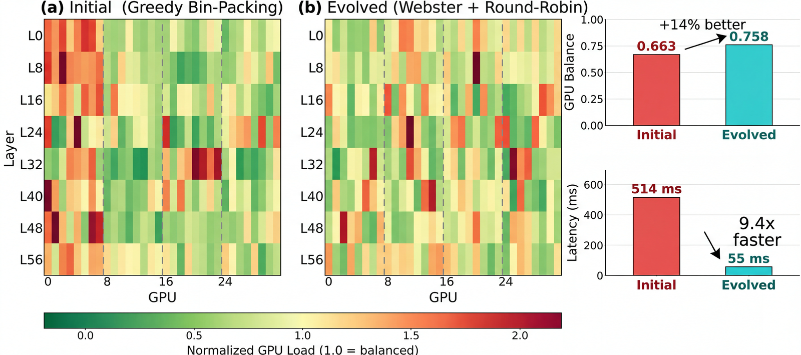
LLM Serving Example: GPU Model Placement for LLM Serving
Problem. Given multiple LLM models and a cluster of GPUs (each with 80 GB memory), the goal is to assign models to GPUs to minimize the maximum KV-cache pressure ratio (KVPR) defined as the ratio of request load to available memory. Lower KVPR indicates reduced GPU bottlenecks, improving serving throughput and stability.
Result. Starting from a naive first-fit packing baseline, EvoX discovers a binary-search + best-fit-decreasing strategy that jointly optimizes model size and request pressure by mapping each model to a combined weight and performing bin packing against a tuned capacity threshold.
Across 50 test scenarios, EvoX achieves a KVPR of 0.0339 (lower is better), improving upon the prior human SOTA (Arxiv’25, KVPR = 0.0479) by 29%, with 100% successful placements across all tests. EvoX also outperforms other frameworks: OpenEvolve (0.0396), GEPA (0.0396), and ShinkaEvolve (0.0396) by 14%.
💡 Best Solution Found
GPU_MEM_SIZE = 80 # GB

# EVOLVE-BLOCK-START

def compute_model_placement(gpu_num, models):
    """Minimize max KVPR via binary search on T. For target T, give each model weight w=a+T*s (a=req_rate/slo, s=size) and each GPU capacity T*M; pack with Best-Fit-Decreasing and return placement for minimal feasible T."""
    M=GPU_MEM_SIZE; EPS=1e-12
    it=[(m, m.req_rate/max(m.slo,EPS), m.model_size) for m in models]
    if any(s>M for _,_,s in it) or sum(s for _,_,s in it)>gpu_num*M:
        raise ValueError("Unable to place model")
    def pack(T,ret=False):
        cap=[T*M]*gpu_num; P=[[] for _ in range(gpu_num)]
        ws=sorted(((m,a+T*s) for m,a,s in it), key=lambda x:x[1], reverse=True)
        for m,w in ws:
            bi=-1; br=float('inf')
            for i in range(gpu_num):
                r=cap[i]-w
                if r>=-1e-12 and r<br:
                    bi=i; br=r
            if bi<0: return None if ret else False
            cap[bi]-=w; P[bi].append(m)
        return {i:P[i]} if ret else True
    hi=1.0; tries=0
    while not pack(hi):
        hi*=2.0; tries+=1
        if tries>60: raise ValueError("Unable to place model")
    lo=0.0
    for _ in range(35):
        mid=(lo+hi)/2.0
        if pack(mid): hi=mid
        else: lo=mid
    res=pack(hi,True)
    if res is None: raise ValueError("Unable to place model")
    return res

# EVOLVE-BLOCK-END

if __name__ == "__main__":
    # Test the algorithm

    from evaluator import generate_test_gpu_models
    from evaluator import calculate_kvcache_pressure
    from evaluator import safe_float
    import numpy as np

    test_cases = generate_test_gpu_models()
    all_kvpr = []
    for i, (gpu_num, gpu_models) in enumerate(test_cases):

        results = compute_model_placement(gpu_num, gpu_models)
        max_kvpr = calculate_kvcache_pressure(results)
        all_kvpr.append(safe_float(max_kvpr))

    avg_kvpr = np.mean(all_kvpr)
    if avg_kvpr != 0:
        avg_kvpr = 1.0 / avg_kvpr

    print(f"Max KVPR: {avg_kvpr:.3f}")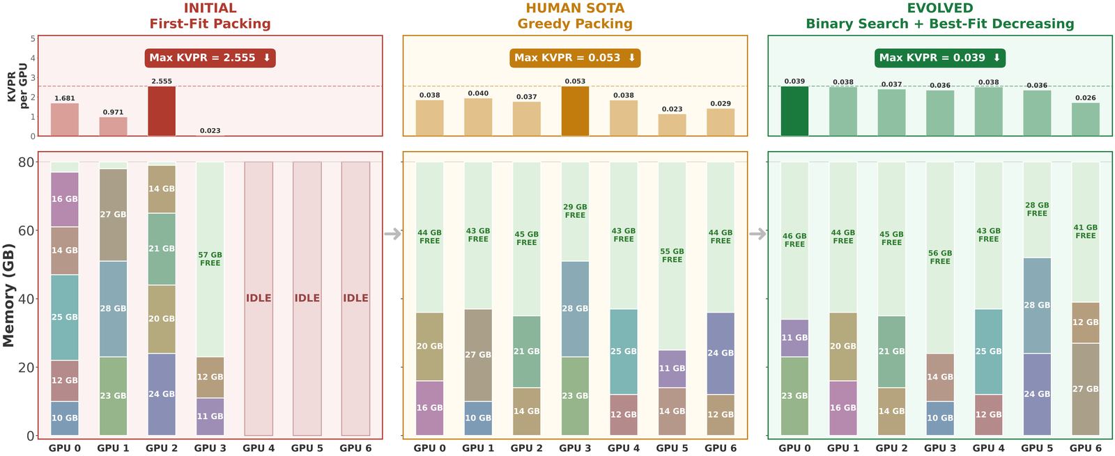
Systems More Example: Multi-Region and Multi-Cloud Data Transfer
Problem. Broadcast a large dataset from a source region to multiple destinations across cloud providers (e.g., AWS, GCP, Azure) under heterogeneous egress pricing. The objective is to minimize total transfer cost while delivering data to all destinations.
Result. Starting from a Dijkstra shortest-path baseline, EvoX learns to construct shared relay trees that reuse intermediate regions across transfers, forming Steiner-like topologies when cost-effective.
On the benchmark setting involving the transfer of 300GB of data from the GCP Singapore region to six cross-cloud destinations, the discovered strategy reduces cost from $1046 to $623 (41% cost reduction). This outperforms OpenEvolve (32%), GEPA (38%, up to 40% with 250+ iterations), and ShinkaEvolve (22%), all evaluated under a fixed budget of 100 iterations.
💡 Best Solution Found
# EVOLVE-BLOCK-START
import networkx as nx
import json
import os
import pandas as pd
from typing import Dict, List

def search_algorithm(src, dsts, G, num_partitions):
    """
    Ensemble Steiner Tree Search with Frequency-Based Candidate Selection.
    1. Preprocessing: Cleans graph, computes APSP, and identifies high-frequency intermediate nodes
       appearing in shortest paths between terminals.
    2. Multi-Start Search: Generates a population of trees using:
       - Deterministic Takahashi-Matsuyama.
       - Randomized Shortest Path Trees (perturbed weights).
    3. Refinement: Applies Iterative MSA to the best candidate sets to optimize the topology.
    4. Selection: Returns the lowest-cost tree found.
    """
    import random
    from collections import Counter

    # 1. Graph Cleanup & Precomputation
    h = G.copy()
    valid_edges = []
    for u, v, d in h.edges(data=True):
        if d.get("cost") is not None and d.get("throughput", 0) > 0:
            valid_edges.append((u, v, d))

    h_clean = nx.DiGraph()
    h_clean.add_edges_from(valid_edges)
    h_clean.add_nodes_from(G.nodes())

    try:
        apsp = dict(nx.all_pairs_dijkstra(h_clean, weight="cost"))
    except:
        return BroadCastTopology(src, dsts, num_partitions)

    if src not in apsp:
        return BroadCastTopology(src, dsts, num_partitions)

    terminals = set(dsts) | {src}

    # 2. Candidate Identification (Frequency Analysis)
    node_freq = Counter()
    terminal_list = list(terminals)
    pairs = []
    if len(terminal_list) > 1:
        for _ in range(100):
            u, v = random.sample(terminal_list, 2)
            if u != v: pairs.append((u, v))

    for u, v in pairs:
        if u in apsp and v in apsp[u][1]:
            path = apsp[u][1][v]
            node_freq.update(path)

    freq_candidates = [n for n, c in node_freq.most_common(20) if n not in terminals]

    best_tree = None
    min_cost = float('inf')

    def get_tree_cost(t):
        return sum(d.get("cost", 0) for _, _, d in t.edges(data=True))

    def refine_candidates(initial_cands):
        curr_cands = set(initial_cands)
        local_best = None
        local_min = float('inf')

        for _ in range(3):
            active = list(terminals | curr_cands)
            metric_g = nx.DiGraph()

            for u in active:
                if u not in apsp: continue
                targets = apsp[u][0]
                for v in active:
                    if u != v and v in targets:
                        metric_g.add_edge(u, v, weight=targets[v])

            if src in metric_g:
                metric_g.remove_edges_from(list(metric_g.in_edges(src)))

            if not metric_g.nodes(): break

            try:
                msa = nx.minimum_spanning_arborescence(metric_g, attr="weight")
            except: break

            leaves = [n for n in msa.nodes() if msa.out_degree(n) == 0 and n not in terminals]
            msa.remove_nodes_from(leaves)

            phys = nx.DiGraph()
            possible = True
            for u, v in msa.edges():
                if u in apsp and v in apsp[u][1]:
                    path = apsp[u][1][v]
                    nx.add_path(phys, path)
                    for x, y in zip(path, path[1:]):
                        if h_clean.has_edge(x, y):
                            phys.add_edge(x, y, **h_clean[x][y])
                        else: possible = False
                else: possible = False

            if not possible: break

            c = get_tree_cost(phys)
            if c < local_min:
                local_min = c
                local_best = phys

            branching = {n for n in phys.nodes() if phys.out_degree(n) > 1}
            new_cands = (branching | set(phys.nodes())) - terminals
            if new_cands.issubset(curr_cands): break
            curr_cands = new_cands

        return local_best, local_min

    # Strategy A: Takahashi-Matsuyama
    tm_cands = set()
    tm_reached = {src}
    tm_unreached = set(dsts) - {src}
    while tm_unreached:
        best_n, best_p, min_d = None, None, float('inf')
        for u in tm_reached:
            if u not in apsp: continue
            for v in tm_unreached:
                if v in apsp[u][0] and apsp[u][0][v] < min_d:
                    min_d = apsp[u][0][v]
                    best_n, best_p = v, u
        if best_n:
            path = apsp[best_p][1][best_n]
            tm_cands.update(path)
            tm_reached.update(path)
            tm_unreached.remove(best_n)
        else: break

    t, c = refine_candidates(tm_cands - terminals)
    if t and c < min_cost:
        min_cost, best_tree = c, t

    # Strategy B: Randomized Perturbation
    for i in range(8):
        perturb = 0.05 + (i * 0.05)
        p_G = nx.DiGraph()
        for u, v, d in h_clean.edges(data=True):
            w = d.get("cost", 0) * random.uniform(1.0 - perturb, 1.0 + perturb)
            p_G.add_edge(u, v, weight=w)

        trial_cands = set(freq_candidates)
        try:
            p_dists, p_paths = nx.single_source_dijkstra(p_G, src, weight="weight")
            for d in dsts:
                if d in p_paths:
                    trial_cands.update(p_paths[d])
        except: pass

        t, c = refine_candidates(trial_cands - terminals)
        if t and c < min_cost:
            min_cost, best_tree = c, t

    bc = BroadCastTopology(src, dsts, num_partitions)
    final = best_tree if best_tree else h_clean

    for dst in dsts:
        if dst == src: continue
        edges = []
        if final.has_node(dst) and nx.has_path(final, src, dst):
            try:
                p = nx.shortest_path(final, src, dst, weight="cost")
                edges = [[u, v, final[u][v]] for u, v in zip(p, p[1:])]
            except: pass

        if not edges and src in apsp and dst in apsp[src][1]:
            p = apsp[src][1][dst]
            edges = [[u, v, h_clean[u][v]] for u, v in zip(p, p[1:])]

        if edges:
            for i in range(num_partitions):
                bc.set_dst_partition_paths(dst, i, edges)

    return bc

class SingleDstPath(Dict):
    partition: int
    edges: List[List]  # [[src, dst, edge data]]

class BroadCastTopology:
    def __init__(self, src: str, dsts: List[str], num_partitions: int = 4, paths: Dict[str, SingleDstPath] = None):
        self.src = src  # single str
        self.dsts = dsts  # list of strs
        self.num_partitions = num_partitions

        # dict(dst) --> dict(partition) --> list(nx.edges)
        # example: {dst1: {partition1: [src->node1, node1->dst1], partition 2: [src->dst1]}}
        if paths is not None:
            self.paths = paths
            self.set_graph()
        else:
            self.paths = {dst: {str(i): None for i in range(num_partitions)} for dst in dsts}

    def get_paths(self):
        print(f"now the set path is: {self.paths}")
        return self.paths

    def set_num_partitions(self, num_partitions: int):
        self.num_partitions = num_partitions

    def set_dst_partition_paths(self, dst: str, partition: int, paths: List[List]):
        """
        Set paths for partition = partition to reach dst
        """
        partition = str(partition)
        self.paths[dst][partition] = paths

    def append_dst_partition_path(self, dst: str, partition: int, path: List):
        """
        Append path for partition = partition to reach dst
        """
        partition = str(partition)
        if self.paths[dst][partition] is None:
            self.paths[dst][partition] = []
        self.paths[dst][partition].append(path)

def make_nx_graph(cost_path=None, throughput_path=None, num_vms=1):
    """
    Default graph with capacity constraints and cost info
    nodes: regions, edges: links
    per edge:
        throughput: max tput achievable (gbps)
        cost: $/GB
        flow: actual flow (gbps), must be < throughput, default = 0
    """
    # Use relative path from this file's location
    current_dir = os.path.dirname(os.path.abspath(__file__))

    if cost_path is None:
        cost = pd.read_csv(os.path.join(current_dir, "profiles/cost.csv"))
    else:
        cost = pd.read_csv(cost_path)

    if throughput_path is None:
        throughput = pd.read_csv(os.path.join(current_dir, "profiles/throughput.csv"))
    else:
        throughput = pd.read_csv(throughput_path)

    G = nx.DiGraph()
    for _, row in throughput.iterrows():
        if row["src_region"] == row["dst_region"]:
            continue
        G.add_edge(row["src_region"], row["dst_region"], cost=None, throughput=num_vms * row["throughput_sent"] / 1e9)

    for _, row in cost.iterrows():
        if row["src"] in G and row["dest"] in G[row["src"]]:
            G[row["src"]][row["dest"]]["cost"] = row["cost"]

    # some pairs not in the cost grid
    no_cost_pairs = []
    for edge in G.edges.data():
        src, dst = edge[0], edge[1]
        if edge[-1]["cost"] is None:
            no_cost_pairs.append((src, dst))
    print("Unable to get costs for: ", no_cost_pairs)

    return G

# EVOLVE-BLOCK-END

# Helper functions that won't be evolved
def create_broadcast_topology(src: str, dsts: List[str], num_partitions: int = 4):
    """Create a broadcast topology instance"""
    return BroadCastTopology(src, dsts, num_partitions)

def run_search_algorithm(src: str, dsts: List[str], G, num_partitions: int):
    """Run the search algorithm and return the topology"""
    return search_algorithm(src, dsts, G, num_partitions)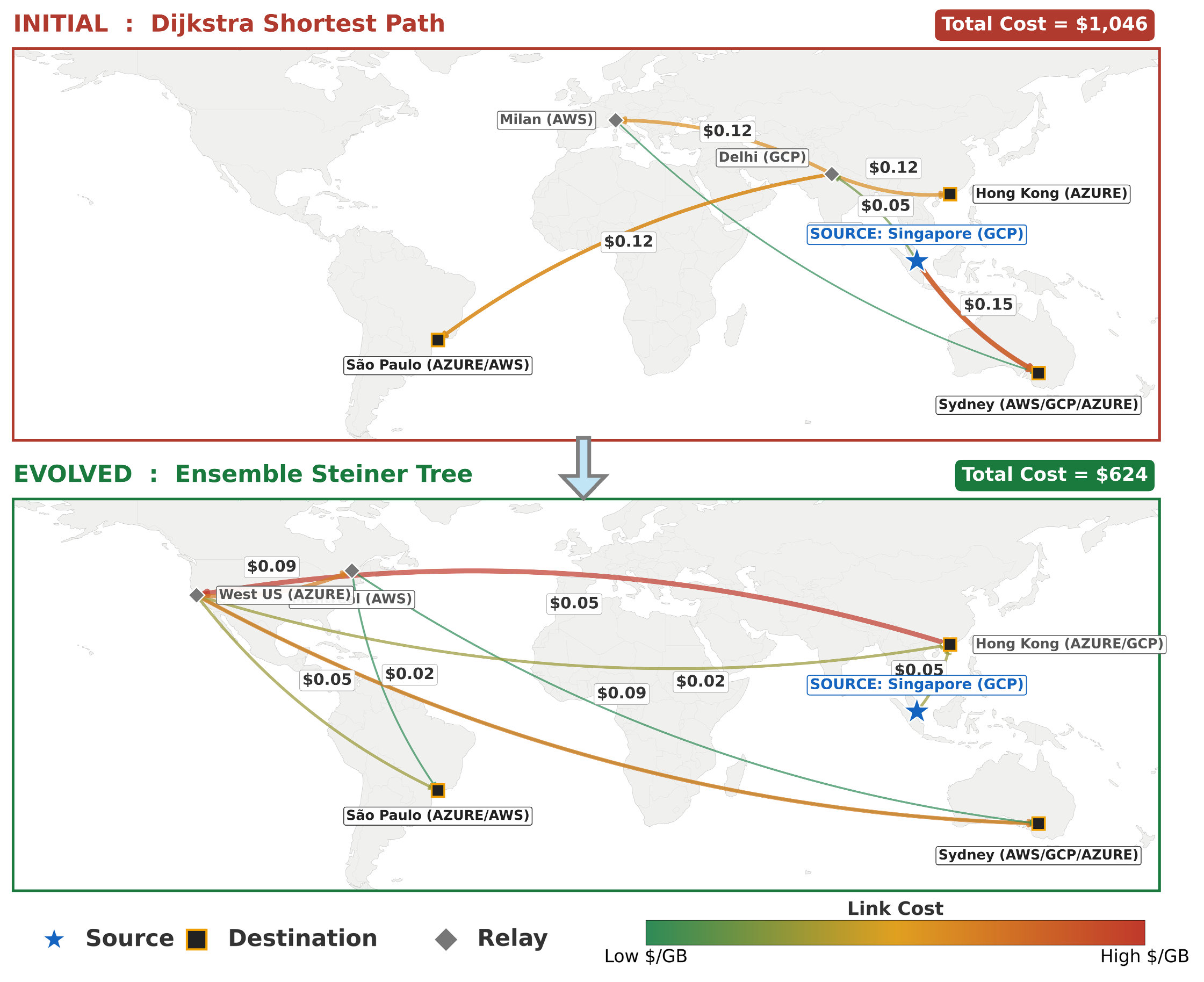
Category 3: Image Generation
Image Example: Generate Sky Festival Image
Problem. This task evaluates whether SkyDiscover can optimize images, not just code or text. Each solution is an image evolved by generating and scoring variants from a candidate pool. The task is a highly constrained floating sky-festival scene. The image depicts a whimsical celebration on a floating island in the sky, with hot-air balloons, shaped clouds, characters, and decorations. However, unlike typical image generation, many details must match exact structural constraints.
Requirements: The system must generate a floating sky-festival image where many details must be correct: 9 clouds with specific shapes, 5 hot-air balloons with exact colors, passengers, and banner text, a floating island with 4 ordered trees, and a party table with precisely counted and colored items. The scene also includes 6 characters with specific attributes (e.g., robot buttons, grandmother’s left-hand thumbs-up), along with animals and a correctly ordered 7-band rainbow.
Setup. Each generated image is graded by a GPT-5 vision judge using a strict rubric. The judge assigns scores across 7 categories — cloud shapes (15), balloons (20), floating island (10), table items (20), characters (15), creatures (10), and lighting (10), for a total of 100 points.
Results. Over 100 iterations, the best score rises from 18/100 → 33/100 as evolution progressively fixes different parts of the scene.
Early candidates often get the vibe right (sunny festival, a few recognizable cloud silhouettes) but miss most hard constraints (missing island structure, wrong balloon passengers, incorrect counts). As the search continues, structure emerges (a floating island with trees, more balloons, clearer cloud shapes), and later iterations begin satisfying previously-missing categories like the banner text and table items, i.e., categories that were frequently near-zero early on.

Category 4: Algorithmic Discovery
Algorithms Example: Polyomino Packing (Frontier-CS)
Problem. We evaluate algorithmic discovery on Frontier-CS, a benchmark of 172 open-ended computer science problems spanning algorithmic optimization and research tasks. We illustrate the evolution process on the first Frontier-CS problem. The goal is to pack every distinct polyomino of sizes 1 through n into a rectangular grid, allowing rotations and reflections, without overlap, while minimizing the total grid area.
Result. Starting from a weak baseline, AdaEvolve discovers increasingly effective packing strategies (e.g., improved placement orderings, symmetry handling, and local compaction), leading to denser fillings and lower-area layouts over iterations.
Usability and Tooling
1️⃣ Simple and Easy-to-Use
SkyDiscover is designed to be plug-and-play. Bring a task (and a way to evaluate it), choose an algorithm, and run.
The same interface lets you (1) apply SkyDiscover to new problems quickly and (2) compare different discovery methods under the same setup — simply by changing a single argument (e.g., search="evox" or search="adaevolve").
from skydiscover import run_discovery

optimized_solution = run_discovery(
    evaluator="evaluator.py",
    search="adaevolve" / "evox",  # gepa, openevolve, shinkaevolve, ...
    model="gpt-5",
    iterations=100
)
This interface also aligns with the “optimize-anything” API used in systems like GEPA. Algorithms implemented in SkyDiscover can therefore be reused within optimize-anything–style workflows, while benefiting from SkyDiscover’s modular architecture and extensible design.
2️⃣ Human-in-the-Loop Monitoring and Control
SkyDiscover supports human-in-the-loop interaction during discovery.
Expert feedback can play an important role in guiding search, particularly when progress stagnates or optimization dynamics shift. To enable this, we provide an interactive UI for monitoring and controlling runs.
In the example below, the search stagnates around iterations 40-50 before resuming improvement after human feedback is introduced. Feedback can be appended to the system prompt, injected as targeted guidance, or reverted when no longer relevant. This design enables human intervention without disrupting the discovery loop.
We invite the community to use, evaluate, and extend SkyDiscover:
- Use SkyDiscover to tackle challenging optimization and discovery problems
- Compare discovery methods within a unified framework
- Implement new algorithms through a simple interface
- Contribute new problems and benchmarks to advance AI-driven discovery
Acknowledgments
This research was supported by gifts from Accenture, AMD, Anyscale, Broadcom Inc., Google, IBM, Intel, Intesa Sanpaolo, Lambda, Mibura Inc, Samsung SDS, and SAP. We also thank Jiarong Xing, Asankhaya Sharma, and Joseph E. Gonzalez for their valuable feedback and discussion.
Citation
If you find SkyDiscover useful in your research, please cite:
@inproceedings{liu2026skydiscover,
  author    = {Liu, Shu and Cemri, Mert and Agarwal, Shubham and Krentsel, Alexander and Naren, Ashwin and Mang, Qiuyang and Li, Zhifei and Gupta, Akshat and Maheswaran, Monishwaran and Cheng, Audrey and Pan, Melissa and Boneh, Ethan and Ramchandran, Kannan and Sen, Koushik and Zaharia, Matei and Dimakis, Alexandros G. and Stoica, Ion},
  title     = {SkyDiscover: A Flexible, Adaptive Framework for AI-Driven Scientific and Algorithmic Discovery},
  booktitle = {Proceedings of the ACM Conference on AI and Agentic Systems},
  series    = {CAIS '26},
  year      = {2026},
  pages     = {1223--1227},
  publisher = {Association for Computing Machinery},
  doi       = {10.1145/3786335.3813221},
  url       = {https://doi.org/10.1145/3786335.3813221}
}